Recurrent Neural Networks (RNN)
A Recurrent Neural Network works on the principle of saving the output of a particular layer and feeding this back to the input in order to predict the output of the layer.
Why not Feed Forward Neural Network?
In a feed-forward network, information flows only in the forward direction, from the input nodes, through the hidden layers (if any), and to the output nodes. There are no cycles or loops in the network.

Decisions are based on current input, No Memory about the past, No future scope. Feed-forward neural networks are used in general regression and classification problems.
Issues in Feed-Forward network:
- Cannot Handle Sequential Data.
- Consider only the current input.
- Cannot memorize previous inputs.
The solution to these issues in Recurrent Neural Network (RNN):
- Can Handle Sequential Data.
- Accepting the current input data and previously received inputs.
- RNNs can memorize previous inputs due to their internal memory.
Below is how you can convert a Feed-Forward Neural Network into a Recurrent Neural Network:

The nodes in different layers of the neural network are compressed to form a single layer of recurrent neural networks. A, B, and C are the parameters of the network.

Here, “x” is the input layer, “h” is the hidden layer, and “y” is the output layer. A, B, and C are the network parameters used to improve the output of the model. At any given time t, the current input is a combination of input at x(t) and x(t-1). The output at any given time is fetched back to the network to improve on the output.

Notations:
h(t)- new state
fc - function with parameter c
h(t-1) - old state
x(t) - input vector at timestamp t
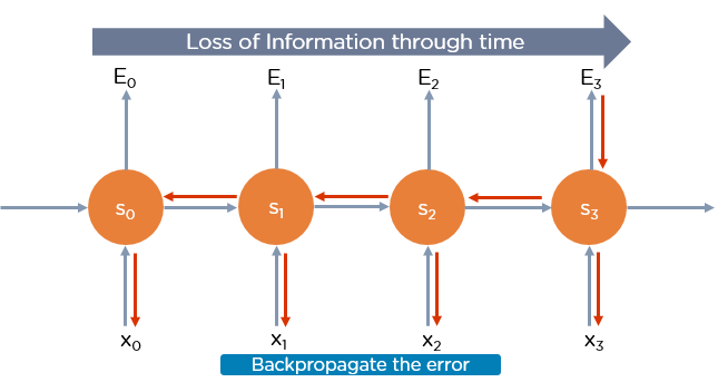
Recurrent Neural Network uses the Backpropagation algorithm, but it is applied for every timestamp. It is known as Backpropagation Through Time.
Backpropagation Through Time (BTT)
The backpropagation learning algorithm is an extension of standard backpropagation that performs gradient descent on an unfolded network.
The gradient descent weight updates have contributions from each timestamp.
The errors have to be back-propagated through time as well as through the network.
Limitations of Backpropagation Through Time:
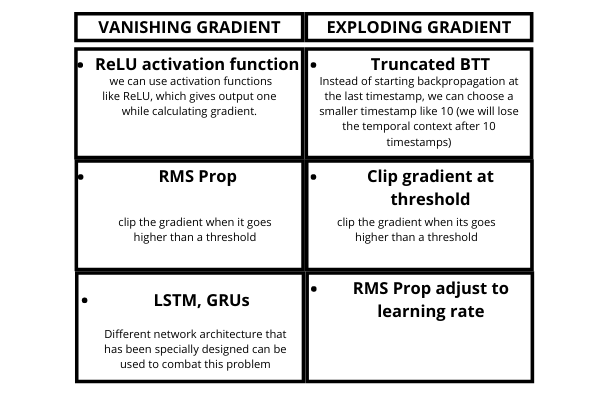
- Vanishing Gradient
- Exploding Gradient
Recurrent Neural Networks enable you to model time-dependent and sequential data problems, such as stock market prediction, machine translation, and text generation. You will find, however, that recurrent Neural Networks are hard to train because of the gradient problem.
Vanishing Gradient Problem
RNNs suffer from the problem of vanishing gradients. The gradients carry information used in the RNN, and when the gradient becomes too small, the parameter updates become insignificant. This makes the learning of long data sequences difficult.
Exploding Gradient Problem
While training a neural network, if the slope tends to grow exponentially instead of decaying, this is called an Exploding Gradient. This problem arises when large error gradients accumulate, resulting in very large updates to the neural network model weights during the training process.
Major Issues in Gradient problems:
- Long Training Time
- Poor Performance
- Bad Accuracy
Overcome these Challenges:
Long Short-Term Memory Networks (LSTM)
Long Short-Term Memory networks are usually just called “LSTMs”.
They are a special kind of Recurrent Neural Networks which are capable of learning long-term dependencies.
What are long-term dependencies?
Many times only recent data is needed in a model to perform operations. But there might be a requirement from data that was obtained in the past.
Let’s look at the following example:
If we are trying to predict the last word in “The clouds are in the sky” we don't need any further context - it's pretty obvious the next word is going to be the sky.
In such cases, where the gap between the relevant information and the place that is needed is small, RNNs can learn to use the past information.
LSTMs are a special kind of Recurrent Neural Network — capable of learning long-term dependencies by remembering information for long periods is the default behavior.
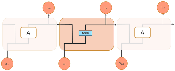
All recurrent neural networks are in the form of a chain of repeating modules of a neural network. In standard RNNs, this repeating module will have a very simple structure, such as a single tanh layer.
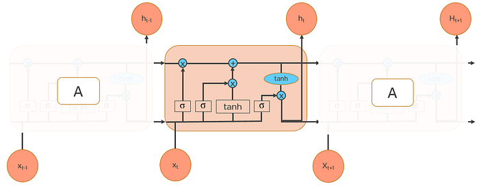
LSTMs also have a chain-like structure, but the repeating module is a bit different structure. Instead of having a single neural network layer, four interacting layers are communicating extraordinarily.
Let's know about some notations and statements:

Cell State — The key to LSTMs is the cell state, the horizontal line running through the top of the diagram.
The cell state is kind of like a conveyor belt. It runs straight down the entire chain, with only some minor linear interactions. It's very easy for information to just flow along with it unchanged.
The LSTM does have the ability to remove or add information to the cell state, carefully regulated by a structure called gates
Gates — Gates are the way to optionally let information through. They are composed out of a sigmoid neural net layer and a pointwise multiplication operation.
The sigmoid layer outputs numbers between zero and one, describing how much of each component should be let through. A value of zero means “let nothing through” while a value of one means “let everything through”
An LSTM has three of these gates, to protect and control the cell state.
Workings of LSTMs
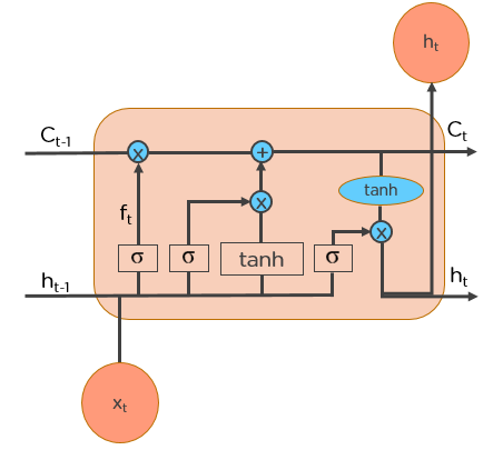
LSTMs work in a 4-step process:
STEP 1:
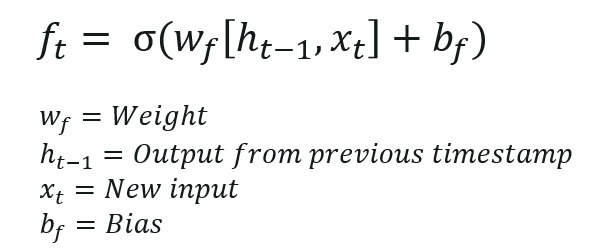
— The first step in our LSTM is to decide which information should be omitted from the cell in that particular timestamp.
— This decision is made by a Sigmoid Layer called the “Forget Gate Layer”.
— It looks at h(t-1) and x(t) and outputs a number between 0 and 1 for each number in the cell state (c t-1).
— 1 represents “completely keep this” while a 0 represents “completely get rid of this”.
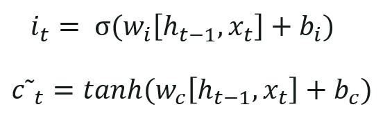
STEP 2:
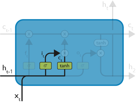
— In this second layer, there are two parts. One is the sigmoid function and the other is the tanh function.
— In the sigmoid function, it decides which value to let through (0 or 1).
— In the tanh function, it gives weightage to the value which is passed, deciding their level of importance (-1 to 1).
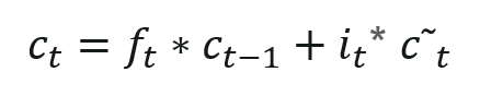
STEP 3:
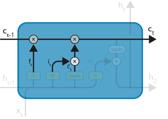
— Now, we will update the old cell state c(t-1), into the new cell c(t). First, we multiply the old state c(t-1) by f(t), forgetting the things we decided to forget earlier.
— Then we add i(t) * c(t). These are the new candidate values, scaled by how much we decided to update each state value.
STEP 4:
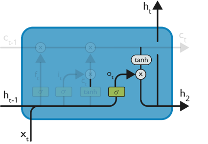
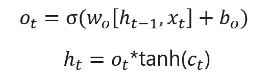
— Finally, we need to decide what we are going to output. This output will be based on our cell state but will be a filtered version.
— We will run a sigmoid layer which decides what parts of the cell state we are going to output. Then, we put the cell state through tanh (push the values to be between −1 and 1) and multiply it by the output of the sigmoid gate, so that we only output the parts we decide to.
Advantages of LSTM:
- Non-decaying error backpropagation
- For long-time lag problems, LSTM can handle noise and continuous values.
- No parameter fine-tuning
- Memory for long time periods.
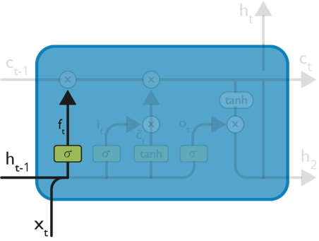
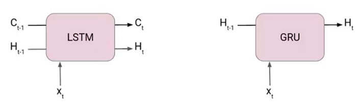
Gated Recurrent Units(GRUs)
A slightly more dramatic variation on the LSTM is the called Recurrent Unit or GRU.
It combines the forget and input gates into a single “update gate”
It also merges the cell state and hidden state and makes some other changes. The resulting model is simple than standard LSTM models and has been growing increasingly popular.
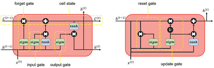
Reset Gate — Short term memory
Update Gate — Long Term memory
LSTM vs GRU
— A GRU has two gates, an LSTM has three gates.
— In GRUs
- No internal memory c(t), different from the exposed hidden state.
- No output gate as in LSTMs
— The input and forget gates of LSTMs are coupled by an update gate in GRUs and the reset gate (GRUs) is applied directly to the previous hidden state.
— GRUs: No non-linearity when computing the output.